
D. Bompadre Rigel S.p.A. (Roma)
In all sectors where it is essential to monitor and control the degree of contamination of production areas, it is necessary to have systems capable of detecting the concentration of particles in the air. The use of OPC (Optical Particle Counters) is still the most widespread means for verifying particle contamination in the pharmaceutical sector, hospital, electronics and food. Very often, however, there is the feeling that there is no total clarity on some concepts of acquisition of particle data. In this article we will describe, albeit briefly, some fundamental aspects for the quality of the data acquired during the production process.
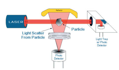 Fig. 1 Principle of laser diffusion of an OPC
The operating logic of an OPC is binary and is based on the use of one or more electrical voltage comparators at which signal counters are associated (see Figure 2).
Fig. 1 Principle of laser diffusion of an OPC
The operating logic of an OPC is binary and is based on the use of one or more electrical voltage comparators at which signal counters are associated (see Figure 2).
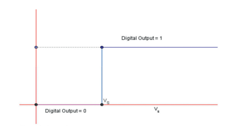 Fig. 2 Operation binary logic graph
In the pharmaceutical field, 2 to 4 signal comparators are usually used, corresponding to the classic nominal particle size diameters such as required by current legislation (see figure 3). When a particle enters the OPC system, passing through the sensitive measurement volume, it will produce a voltage signal Vp.
Fig. 2 Operation binary logic graph
In the pharmaceutical field, 2 to 4 signal comparators are usually used, corresponding to the classic nominal particle size diameters such as required by current legislation (see figure 3). When a particle enters the OPC system, passing through the sensitive measurement volume, it will produce a voltage signal Vp.
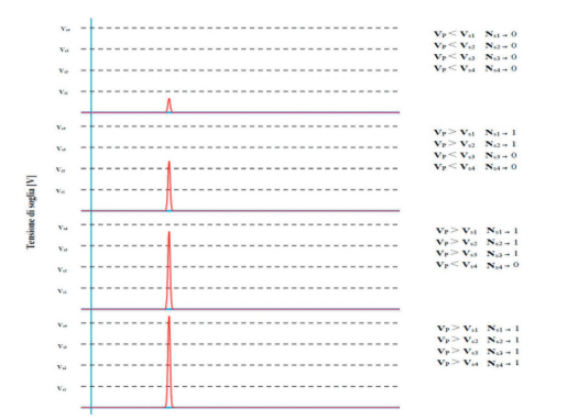 Fig. 3 Update chart of the internal counters of an OPC
The total number of particles sampled during the operating time will subsequently be referred to as Np (total population of particles). The transit of each subsequent sampled particle will be indicated by the updating of a hypothetical counter, Np = Np + 1, like the usual updating logic used in the programming language. Each signal is analyzed through the system of K comparators. The following binary operating logic applies to each comparator:
Vp>Vs → 1 [Ns=Ns+1]
(the signal is recorded; the associated counter is updated)
Vp<Vs → 0 [Ns=Ns]
(the signal is not recorded; the associated counter remains unchanged)
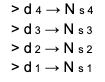
at the end of each operating cycle in which the system has collected Np particles we will have the following situation for the 4 counters:
Fig. 3 Update chart of the internal counters of an OPC
The total number of particles sampled during the operating time will subsequently be referred to as Np (total population of particles). The transit of each subsequent sampled particle will be indicated by the updating of a hypothetical counter, Np = Np + 1, like the usual updating logic used in the programming language. Each signal is analyzed through the system of K comparators. The following binary operating logic applies to each comparator:
Vp>Vs → 1 [Ns=Ns+1]
(the signal is recorded; the associated counter is updated)
Vp<Vs → 0 [Ns=Ns]
(the signal is not recorded; the associated counter remains unchanged)
at the end of each operating cycle in which the system has collected Np particles we will have the following situation for the 4 counters:
 the
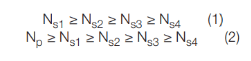
the  condition occurs whenever in the sampled population there are particles with a diameter lower than the minimum sensitive threshold (Vs1) of an OPC. Relation (1) provides a representation of the particle size distribution in the size range> d1 in 4 operating ranges:
 From relation (2) we obtain one of the fundamental parameters that characterize the operation of an OPC, that is the relations
  that are definitive with the term Count Efficiency, where:
Nsk indicates the number of signals (number of particles) that exceed the threshold level Vsk (threshold diameter ds) with respect to the total number of sampled particles Np.
that are definitive with the term Count Efficiency, where:
Nsk indicates the number of signals (number of particles) that exceed the threshold level Vsk (threshold diameter ds) with respect to the total number of sampled particles Np.
 Where:
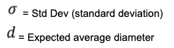
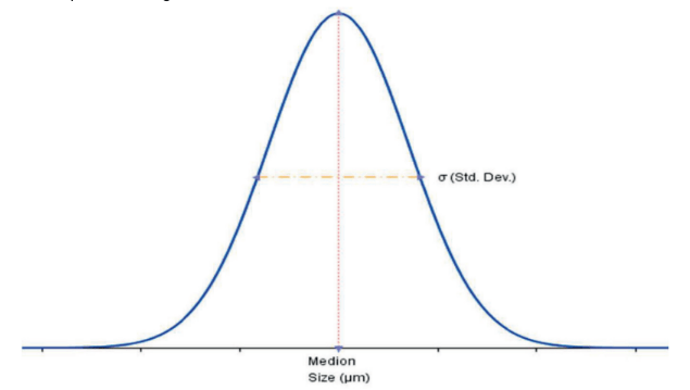 Fig. 4 Particle size distribution of the standard
It is evident that the value of the average diameter of the distribution, which represents the reference diameter, is by symmetry the element of separation between the particle belonging to the standard population having a diameter greater than the average value (
Fig. 4 Particle size distribution of the standard
It is evident that the value of the average diameter of the distribution, which represents the reference diameter, is by symmetry the element of separation between the particle belonging to the standard population having a diameter greater than the average value ( ) and those having a diameter smaller than it .
 When a standard atmosphere generated with the reference population is transferred to the OPC, signals with voltage values Vp will be generated. Consequently we will have at our disposal a population of Vp signals associated with the population of sampled particles.
The distribution of the population Vp is also a population of values of voltage to which it is possible to attribute a value of the median
When a standard atmosphere generated with the reference population is transferred to the OPC, signals with voltage values Vp will be generated. Consequently we will have at our disposal a population of Vp signals associated with the population of sampled particles.
The distribution of the population Vp is also a population of values of voltage to which it is possible to attribute a value of the median  and a standard deviation
  .
The voltage value to be associated with the nominal diameter of the standard population is therefore the value associated with the median of the signal distribution obtained. Indeed, it is observed that the number of signals higher than the chosen threshold value (Vs) is exactly
.
The voltage value to be associated with the nominal diameter of the standard population is therefore the value associated with the median of the signal distribution obtained. Indeed, it is observed that the number of signals higher than the chosen threshold value (Vs) is exactly  , and coincides with the number of signals with a value lower than Vs, this in perfect agreement with the fact that the population of reference particles has a symmetrical distribution with respect to the nominal value medium.
 With this method it is therefore possible to determine the Vs values of the comparators, relative to the threshold diameters present in an OPC under examination.
Resolution
In quantitative terms, the real dispersion of the signals is strongly influenced by the qualitative characteristics of the OPC.
Therefore instruments with different performances (particle size resolution) will show potentially different dispersions.
The operating parameter (R%) quantifies the “Size Resolution” and is described by the following relationship:
With this method it is therefore possible to determine the Vs values of the comparators, relative to the threshold diameters present in an OPC under examination.
Resolution
In quantitative terms, the real dispersion of the signals is strongly influenced by the qualitative characteristics of the OPC.
Therefore instruments with different performances (particle size resolution) will show potentially different dispersions.
The operating parameter (R%) quantifies the “Size Resolution” and is described by the following relationship:
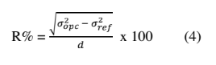 where
where
 Denotes the variance associated with instrumental response when solicited by a monodisperse standard with variance
  values
 Represents the value of the particle diameter associated with the standard.
Figure 5 shows the particle distributions of three OPCs with different resolution values when stressed from the same reference population.
Once the concept of resolution has been defined, it is important to analyze the response of the OPCs in operating conditions and to deepen the link with their Count Efficiency.
Represents the value of the particle diameter associated with the standard.
Figure 5 shows the particle distributions of three OPCs with different resolution values when stressed from the same reference population.
Once the concept of resolution has been defined, it is important to analyze the response of the OPCs in operating conditions and to deepen the link with their Count Efficiency.
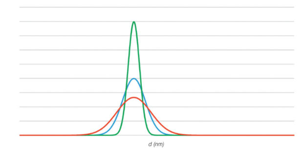 Fig. 5 Comparison chart between OPCs with different resolution values
Count Efficiency
To analyze the instrumental response of OPCs with different resolution values, consider using three OPCs with the following characteristics:
– The first has an excellent resolution (typically this instrumentation is used as an OPC reference during the calibration phases in the laboratory).
– The second and third, representative of two OPCs typically used in the operating range but with significantly different resolutions.
For simplicity we consider the OPC2 and OPC3 equipped with 2 operating thresholds, Vs1 and Vs2 corresponding to two diameters ds1 and ds2. In addition to the two trip thresholds coinciding with the diameters ds1 and ds2, the OPC1 also has an operating threshold ds0 such that ds0 <<ds1, so that it can be used as a reference.
As a first case, we analyze the instrumental response of the three OPCs when using standard monodisperse populations, with nominal diameter the associated values match exactly at the threshold d2 of the three OPC examined.
Figure 6 also shows the counts of the counters with the related Count Efficiency values.
Fig. 5 Comparison chart between OPCs with different resolution values
Count Efficiency
To analyze the instrumental response of OPCs with different resolution values, consider using three OPCs with the following characteristics:
– The first has an excellent resolution (typically this instrumentation is used as an OPC reference during the calibration phases in the laboratory).
– The second and third, representative of two OPCs typically used in the operating range but with significantly different resolutions.
For simplicity we consider the OPC2 and OPC3 equipped with 2 operating thresholds, Vs1 and Vs2 corresponding to two diameters ds1 and ds2. In addition to the two trip thresholds coinciding with the diameters ds1 and ds2, the OPC1 also has an operating threshold ds0 such that ds0 <<ds1, so that it can be used as a reference.
As a first case, we analyze the instrumental response of the three OPCs when using standard monodisperse populations, with nominal diameter the associated values match exactly at the threshold d2 of the three OPC examined.
Figure 6 also shows the counts of the counters with the related Count Efficiency values.
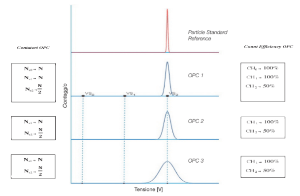 Fig. 6 Comparison chart between OPCs on the second threshold
As expected, the results of the 3 OPCs at the end of the sampling will be completely equivalent. The first channel of the OPCs (2 and 3) will provide a value of Ns1 equal to N, the same response will also be given by the CH0 and CH1 channels of the OPC 1 reference (Count Efficiency = 100%) as the population of the sample used will generate on the three OPC voltage signals Vp always greater than the threshold value Vs1. As for the results relating to the second channel of the three OPCs, they will coincide with .
In fact, represents the number of particles of the standard having a diameter greater than the nominal diameter. (See Size Calibration).
In Figure 7 the same considerations are made as in the previous case, using a reference population having a nominal diameter of particles exactly coinciding with the threshold diameter d1.
Figure 7 also shows the counts of the counters with the related Count Efficiency values.
Fig. 6 Comparison chart between OPCs on the second threshold
As expected, the results of the 3 OPCs at the end of the sampling will be completely equivalent. The first channel of the OPCs (2 and 3) will provide a value of Ns1 equal to N, the same response will also be given by the CH0 and CH1 channels of the OPC 1 reference (Count Efficiency = 100%) as the population of the sample used will generate on the three OPC voltage signals Vp always greater than the threshold value Vs1. As for the results relating to the second channel of the three OPCs, they will coincide with .
In fact, represents the number of particles of the standard having a diameter greater than the nominal diameter. (See Size Calibration).
In Figure 7 the same considerations are made as in the previous case, using a reference population having a nominal diameter of particles exactly coinciding with the threshold diameter d1.
Figure 7 also shows the counts of the counters with the related Count Efficiency values.
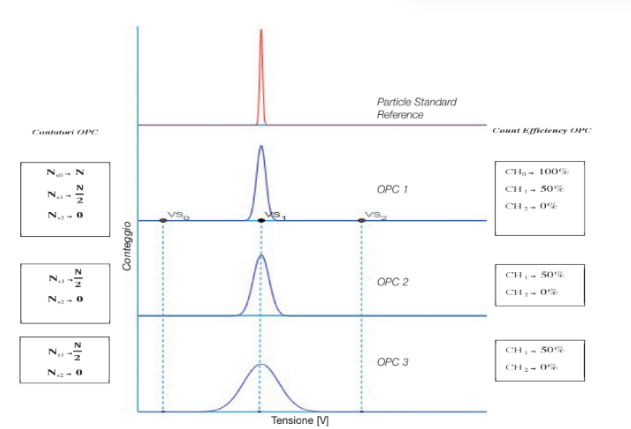 Fig. 7 Comparison chart between OPCs on the first threshold
The CH1 channels of the three OPCs will provide values Ns1 equal to and the Count Efficiency will be equal to 50% for the three OPT considered.
In fact Vs1 coincides with the median of the signals generated by the reference population, as already highlighted on the threshold examined previously. It is useful to note that the CH0 channel corresponding to the threshold Vs0 of the OPC 1 reference gives N.
In fact, the standard monodisperse population used with average diameter d1 generates Vp values which are always and in any case greater than the threshold value Vs0. For this reason it is possible to consider the OPC1 as a reference, as it is able to provide the real data of the population N of particles present in the reference population used with nominal diameter d1. For this reason, the calculation of the Count Efficiency is carried out using for N the value Ns0 relating to a reference OPC.
It is important to go at this point to go analyze the expected response of the three OPCs, when the monodisperse populations used to generate the standard atmospheres have mean diameter values that differ from the threshold value. In particular, two distinct operating conditions can be considered:
Fig. 7 Comparison chart between OPCs on the first threshold
The CH1 channels of the three OPCs will provide values Ns1 equal to and the Count Efficiency will be equal to 50% for the three OPT considered.
In fact Vs1 coincides with the median of the signals generated by the reference population, as already highlighted on the threshold examined previously. It is useful to note that the CH0 channel corresponding to the threshold Vs0 of the OPC 1 reference gives N.
In fact, the standard monodisperse population used with average diameter d1 generates Vp values which are always and in any case greater than the threshold value Vs0. For this reason it is possible to consider the OPC1 as a reference, as it is able to provide the real data of the population N of particles present in the reference population used with nominal diameter d1. For this reason, the calculation of the Count Efficiency is carried out using for N the value Ns0 relating to a reference OPC.
It is important to go at this point to go analyze the expected response of the three OPCs, when the monodisperse populations used to generate the standard atmospheres have mean diameter values that differ from the threshold value. In particular, two distinct operating conditions can be considered:
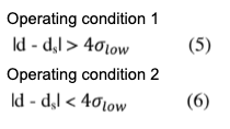
 is the Std Dev associated with the OPC with the lowest resolution (OPC3)
If the relation 5 is valid, the chosen diameters are sufficiently far from the threshold diameters and therefore from the population of the signals generated in the three OPCs will give a Count Efficiency response equal to 0% when all the signals Vp are lower than Vs (ds – d> 4 ) and equal to 100% when all the signals Vp are greater than Vs (d – ds> 4 ).
Therefore, if the mean diameter of the standard population is sufficiently less than the threshold diameter (relation 5), the relative Count Efficiency results equal to 0%, when the average diameter of the standard corresponds exactly to the threshold diameter, the Count Efficiency is equal to 50% and reaches the value of 100% only when the average diameter of the population is sufficiently greater than the diameter threshold.
Figure 8 shows the typical Count Efficiency curves relating to the three OPCs under consideration.
is the Std Dev associated with the OPC with the lowest resolution (OPC3)
If the relation 5 is valid, the chosen diameters are sufficiently far from the threshold diameters and therefore from the population of the signals generated in the three OPCs will give a Count Efficiency response equal to 0% when all the signals Vp are lower than Vs (ds – d> 4 ) and equal to 100% when all the signals Vp are greater than Vs (d – ds> 4 ).
Therefore, if the mean diameter of the standard population is sufficiently less than the threshold diameter (relation 5), the relative Count Efficiency results equal to 0%, when the average diameter of the standard corresponds exactly to the threshold diameter, the Count Efficiency is equal to 50% and reaches the value of 100% only when the average diameter of the population is sufficiently greater than the diameter threshold.
Figure 8 shows the typical Count Efficiency curves relating to the three OPCs under consideration.
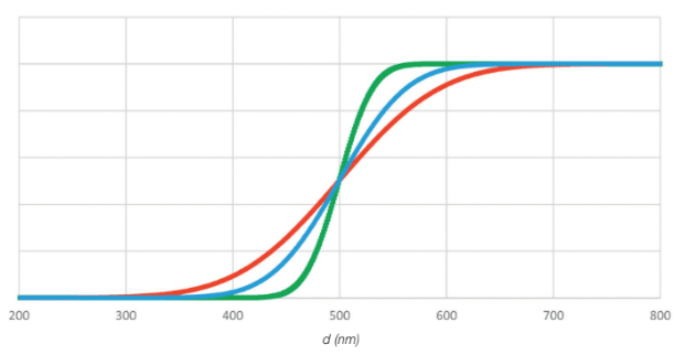 Fig. 8 Representation curve of the counting efficiency between different OPCs
The graph shows how, near the threshold values (validity of relation 6) the response in the Count Efficiency in the three OPCs is substantially different. As expected, the higher the instrumental resolution, the steeper the counting efficiency representation curve near the threshold diameter ds.
Threshold Accuracy Tuning
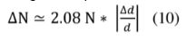
An important aspect in the calibration phase concerns the accuracy in determining the threshold values. The reference standard indicates the acceptability levels of the Count Efficiency values, which on the first threshold are between 30% and 70%. (The nominal reference value is 50%). The Count Efficiency function around the threshold diameter is defined by the characteristic curve shown in figure (9). In fact it is simply a definite function of the variance .
Observing the Count Efficiency characterization curves relating to the three OPCs (Figure 9), it can be seen that the acceptability range between 30 and 70% for Count Efficiency produces an uncertainty in the classification of dynamometers up to 0,5 R.
This uncertainty is to be considered absolutely acceptable within the scope of application of the OPC sensors in the operating field.
Fig. 8 Representation curve of the counting efficiency between different OPCs
The graph shows how, near the threshold values (validity of relation 6) the response in the Count Efficiency in the three OPCs is substantially different. As expected, the higher the instrumental resolution, the steeper the counting efficiency representation curve near the threshold diameter ds.
Threshold Accuracy Tuning
An important aspect in the calibration phase concerns the accuracy in determining the threshold values. The reference standard indicates the acceptability levels of the Count Efficiency values, which on the first threshold are between 30% and 70%. (The nominal reference value is 50%). The Count Efficiency function around the threshold diameter is defined by the characteristic curve shown in figure (9). In fact it is simply a definite function of the variance .
Observing the Count Efficiency characterization curves relating to the three OPCs (Figure 9), it can be seen that the acceptability range between 30 and 70% for Count Efficiency produces an uncertainty in the classification of dynamometers up to 0,5 R.
This uncertainty is to be considered absolutely acceptable within the scope of application of the OPC sensors in the operating field.
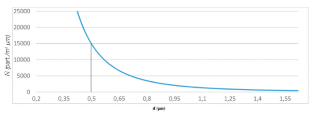 Fig. 9 Particle distribution N
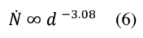 From which we can derive the total concentration relative to a particle size interval such that dp> d
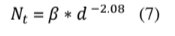 Relation (7) can be used to determine the limits of particle contamination classes in defined clean rooms as ISO 14644-1 / 2 classes when we consider for ß the relation:
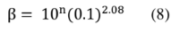 Where n represents the ISO class number (1 ÷ 9).
The relation (7) can therefore be expressed by:
Where n represents the ISO class number (1 ÷ 9).
The relation (7) can therefore be expressed by:
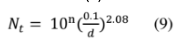 To evaluate the error in determining the threshold relative to a reference diameter (for example the threshold of 0.5 µm) it is useful to quantitatively express the variation ∆N in the number of counts observed with respect to the variation ∆d, between the actual threshold diameter and the assigned one. This quantitative relation is obtained by deriving the relation (9), from which we can estimate in finite terms ∆N through the expression:
 Relation (10) is obviously valid provided that
  «1
For example, when reporting a limiting distribution in an ISO5 class, the threshold level set for this class is 3520 particles> 0.5 µm. A variation ∆d in the determination of the threshold diameter equal to 2% (0.49um ÷ 0.51um), determines a relative percentage change
«1
For example, when reporting a limiting distribution in an ISO5 class, the threshold level set for this class is 3520 particles> 0.5 µm. A variation ∆d in the determination of the threshold diameter equal to 2% (0.49um ÷ 0.51um), determines a relative percentage change  % in number of counts of about 4% (see fig. 10). To evaluate, however, how much the resolution value can influence the determination of the number of particles associated with a specific particle size range of interest, it is necessary to investigate the behavior of the OPC immediately around the threshold diameter. It should in fact be remembered that the Count Efficiency for particles having a diameter equal to the nominal threshold diameter is equal to 50%, and passes respectively to 0 or 100% when passing to diameters sufficiently lower or higher than the threshold one. This transition will be steeper the higher the degree of instrumental resolution. In the real field, if
 is the environmental distribution, the distribution “seen” by the
  tool will simply be given by the relation:
 Figures 9 and 10 show the typical distributions Ṅ and Ṅopc in the limiting case of an ISO5 class for particles> 0.5 µm.
 Fig. 10 Count Efficiency > 0.5 um OPC with 10% resolution
Two zones are identified in the graph (see figure 11) which represent the operating conditions of Undercounting and Overcounting. If the particle distribution were constant around the threshold diameter, the Overcounting or Undercounting errors could be considered balanced and therefore not actually relevant in the particle size classification.
But considering that the particle size distribution in clean rooms is inversely proportional to the powers of d, the overall error leads to a count that is higher the lower the resolution of an OPC.
In Figure 11, an OPT with a resolution equal to 10% was considered, therefore the concentration determined in the ISO5 limit class for particles> 0.5 µm, resulting would be 3643 units / m3 compared to the nominal value of 3520 units / m3, it would result therefore an error in percentage terms, of about 4%.
Fig. 10 Count Efficiency > 0.5 um OPC with 10% resolution
Two zones are identified in the graph (see figure 11) which represent the operating conditions of Undercounting and Overcounting. If the particle distribution were constant around the threshold diameter, the Overcounting or Undercounting errors could be considered balanced and therefore not actually relevant in the particle size classification.
But considering that the particle size distribution in clean rooms is inversely proportional to the powers of d, the overall error leads to a count that is higher the lower the resolution of an OPC.
In Figure 11, an OPT with a resolution equal to 10% was considered, therefore the concentration determined in the ISO5 limit class for particles> 0.5 µm, resulting would be 3643 units / m3 compared to the nominal value of 3520 units / m3, it would result therefore an error in percentage terms, of about 4%.
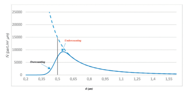 Fig. 11 Particle distribution N and Nopc distribution
The concept of “count efficiency” in optical particle counters
In paragraph 2, ISO 21501-4, reference guide for the verification and calibration methodology of an OPC, defines the concept of count efficiency, as the ratio between the measurements of an OPC compared to a primary reference, using the same reference population (2 Term and definitions – 2.2. Count efficiency – Ratio of the measured result of a light scattering particle counter (LSAPC) to that of an instrument reference using the same sample). The legislation – in paragraph 3 – defines also the limits of acceptance of the values of count efficiency when using populations of certified reference particles (NIST), having nominal diameters corresponding to the values of the first and second operational threshold of the OPC in examination: – (50 ± 20)% On the first threshold corresponding to the lower detection limit. – (100 ± 10)%. On the threshold equal to 1.5 ÷ 2 times the value of the first. (3.3. Count Efficiency – The count efficiency shall be (50±20)% for calibration particles with a size close to the minimum detectable size, and it shall be (100±10)% for calibration particle with a size of 1,5 times to 2 times larger than the minimum detectable particle size). The definition of Count Efficiency at 50% on the first detectable threshold can raise doubts about the not particularly high performance of the OPCs near the lower threshold levels. We will clarify this later, describing the whole process of calibration and analysis of the instrumental response in a real environment.Operating principle of an OPC
An OPC (Optical Particle Counter) is an instrument designed to obtain information on both the number and the particle size distribution of particles dispersed in a transport fluid (liquid or gas), in the particle size range greater than 0.1 µm. The technique used by the OPC instrumentation is based on physics laws that regulate the interaction between light radiation and particles (Mie Scattering). In an OPC, a sample containing airborne particles is passed through the sensing volume measure on which is affected by a focused bright radiation. The interaction between the light radiation and the passing particle produces a diffuse light radiation whose intensity is converted into an electrical signal with an amplitude proportional to the energy associated with the scattering process. If spherical particles with homogeneous optical properties are considered, the values of the signals associated with the scattering process can in principle be biunivocally associated with the diameter of the detected particles. For example, having chosen a reference voltage value which we will indicate as the threshold value Vs, it will correspond to a value of particle diameter ds. Particles with diameter dp> ds, theoretically will be able to produce signals Vp> Vs. It thus becomes possible to use this technique to define a granulometric classification system (see figure 1).
Fig. 1 Principle of laser diffusion of an OPC
The operating logic of an OPC is binary and is based on the use of one or more electrical voltage comparators at which signal counters are associated (see Figure 2).
Fig. 2 Operation binary logic graph
In the pharmaceutical field, 2 to 4 signal comparators are usually used, corresponding to the classic nominal particle size diameters such as required by current legislation (see figure 3). When a particle enters the OPC system, passing through the sensitive measurement volume, it will produce a voltage signal Vp.
Fig. 3 Update chart of the internal counters of an OPC
The total number of particles sampled during the operating time will subsequently be referred to as Np (total population of particles). The transit of each subsequent sampled particle will be indicated by the updating of a hypothetical counter, Np = Np + 1, like the usual updating logic used in the programming language. Each signal is analyzed through the system of K comparators. The following binary operating logic applies to each comparator:
Vp>Vs → 1 [Ns=Ns+1]
(the signal is recorded; the associated counter is updated)
Vp<Vs → 0 [Ns=Ns]
(the signal is not recorded; the associated counter remains unchanged)
at the end of each operating cycle in which the system has collected Np particles we will have the following situation for the 4 counters:
the
From relation (2) we obtain one of the fundamental parameters that characterize the operation of an OPC, that is the relations Size Calibration, Resolution, Count Efficiency and Threshold Accuracy tuning of an OPC using Microsphere reference (setting of the median threshold and verification of accuracy)
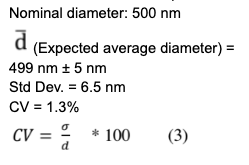
Size Calibration Considering an operational OPC, the first fundamental point is to determine the threshold voltage values Vs in correspondence with the defined particle diameters (ds) of interest. The approach consists in having standards of highly monodisperse particles (the maximum coefficient of variation – CV – relative to the particle size distribution is found to be of a few percentage points). For example, one of the standards used for this application is that of certified reference for latex microspheres. A typical example is shown below of the standard reference population (see figure 4). Particle Reference Example:
Where:
Fig. 4 Particle size distribution of the standard
It is evident that the value of the average diameter of the distribution, which represents the reference diameter, is by symmetry the element of separation between the particle belonging to the standard population having a diameter greater than the average value (
When a standard atmosphere generated with the reference population is transferred to the OPC, signals with voltage values Vp will be generated. Consequently we will have at our disposal a population of Vp signals associated with the population of sampled particles.
The distribution of the population Vp is also a population of values of voltage to which it is possible to attribute a value of the median
With this method it is therefore possible to determine the Vs values of the comparators, relative to the threshold diameters present in an OPC under examination.
Resolution
In quantitative terms, the real
where
Fig. 5 Comparison chart between OPCs with different resolution values
Count Efficiency
To analyze the instrumental response of OPCs with different resolution values, consider using three OPCs with the following characteristics:
– The first has an excellent resolution (typically this instrumentation is used as an OPC reference during the calibration phases in the laboratory).
– The second and third, representative of two OPCs typically used in the operating range but with significantly different resolutions.
For simplicity we consider the OPC2 and OPC3 equipped with 2 operating thresholds, Vs1 and Vs2 corresponding to two diameters ds1 and ds2. In addition to the two trip thresholds coinciding with the diameters ds1 and ds2, the OPC1 also has an operating threshold ds0 such that ds0 <<ds1, so that it can be used as a reference.
As a first case, we analyze the instrumental response of the three OPCs when using standard monodisperse populations, with nominal diameter the associated values match exactly at the threshold d2 of the three OPC examined.
Figure 6 also shows the counts of the counters with the related Count Efficiency values.
Fig. 6 Comparison chart between OPCs on the second threshold
As expected, the results of the 3 OPCs at the end of the sampling will be completely equivalent. The first channel of the OPCs (2 and 3) will provide a value of Ns1 equal to N, the same response will also be given by the CH0 and CH1 channels of the OPC 1 reference (Count Efficiency = 100%) as the population of the sample used will generate on the three OPC voltage signals Vp always greater than the threshold value Vs1. As for the results relating to the second channel of the three OPCs, they will coincide with
Fig. 7 Comparison chart between OPCs on the first threshold
The CH1 channels of the three OPCs will provide values Ns1 equal to
Fig. 8 Representation curve of the counting efficiency between different OPCs
The graph shows how, near the threshold values (validity of relation 6) the response in the Count Efficiency in the three OPCs is substantially different. As expected, the higher the instrumental resolution, the steeper the counting efficiency representation curve near the threshold diameter ds.
Threshold Accuracy Tuning
An important aspect in the calibration phase concerns the accuracy in determining the threshold values. The reference standard indicates the acceptability levels of the Count Efficiency values, which on the first threshold are between 30% and 70%. (The nominal reference value is 50%). The Count Efficiency function around the threshold diameter is defined by the characteristic curve shown in figure (9). In fact it is simply a definite function of the variance
Fig. 9 Particle distribution N
Performance considerations of an OPC in a real environment (clean room)
When operating in a real environment it is necessary to remember that it is not possible to discuss monodisperse particles to which it is given a certain nominal diameter, but a continuous particle size distribution in the whole range considered, between a few nanometers up to a few tens of micron. Depending on the type of operating environment, outdoor, clean room, etc. typical particle size distributions are determined. In clean rooms, the typical particle size distribution is that which can be expressed in the form of power of particle diameter:
To evaluate the error in determining the threshold relative to a reference diameter (for example the threshold of 0.5 µm) it is useful to quantitatively express the variation ∆N in the number of counts observed with respect to the variation ∆d, between the actual threshold diameter and the assigned one. This quantitative relation is obtained by deriving the relation (9), from which we can estimate in finite terms ∆N through the expression:
Figures 9 and 10 show the typical distributions Ṅ and Ṅopc in the limiting case of an ISO5 class for particles> 0.5 µm.
Fig. 10 Count Efficiency > 0.5 um OPC with 10% resolution
Two zones are identified in the graph (see figure 11) which represent the operating conditions of Undercounting and Overcounting. If the particle distribution were constant around the threshold diameter, the Overcounting or Undercounting errors could be considered balanced and therefore not actually relevant in the particle size classification.
But considering that the particle size distribution in clean rooms is inversely proportional to the powers of d, the overall error leads to a count that is higher the lower the resolution of an OPC.
In Figure 11, an OPT with a resolution equal to 10% was considered, therefore the concentration determined in the ISO5 limit class for particles> 0.5 µm, resulting would be 3643 units / m3 compared to the nominal value of 3520 units / m3, it would result therefore an error in percentage terms, of about 4%.
Fig. 11 Particle distribution N and Nopc distribution